SICP
SICP 1.2.3 Solutions
August 30, 2012 19:44
Ex 1.14
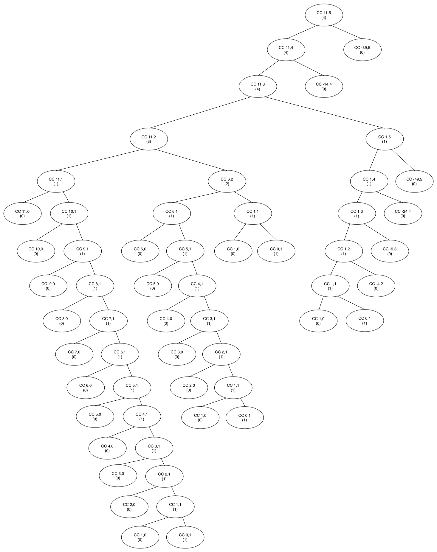
The first part, namely the graph, is fairly easy to produce, if a bit tedious. Simply go through each part of the procedure and add to the tree whenever there is a new call to cc. Naturally I did this by hand on paper first, but I’ve provided a more readable version below.
It’s the second part of the question that gets complicated. Figuring out the order of an algorithm, even a relatively straightforward one like the change-counting one seen here, takes a fair amount of insight; proving it is an even tougher task. Even here, where I’m going to go on at some length, I won’t be fully proving it. What I provide will hopefully be convincing enough, and as I haven’t seen this approach before, it might help in understanding the problem in a different way.
In the following, I’m using n for the amount and k for the number of coin types. For practical purposes, the amount is likely to be more than the number of coin denominations, so it’s assumed that n > k, or in other words that k doesn’t matter that much. One reason why Big-O is used so often that I didn’t get into last time is that it can help reduce the number of variables it’s necessary to consider. Usually there is only one critical value to use in comparing algorithms, ideally in simple expressions. Using Big-O can avoid the need to include what might be distracting variables, since often the behavior when only that critical value increases is what’s important. Our n is the most important value here, as it’s the one likely to grow large.
The order in space actually isn’t too hard to figure. Each call takes up its own space, and spawns at most two branches. Each branch increases the depth of the tree while reducing the amount n , and may also add a branch while reducing k. Considering that n is the most important value, it will be the depth of the tree with n decreasing that matters most for space concerns. Since reducing the amount by 1 increases the depth by 1, the depth grows linearly with n. Thus the order in space is O(n).
For time, we can say that each call to cc takes roughly the same amount of time; there is very little calculation involved otherwise. If addition were expensive, this might be different, but for numbers it really isn’t. We’ll assume it’s the number of procedure calls that determine the order in time.
As I mentioned I won’t do a general proof. Instead I’m going to show it for a specific subset of the problem, and suggest that it applies to all other versions as well.
Imagine a ‘worst-case’ run of the procedure, in which all possible coins are considered as change, and we run through all values from n down to 0.
Such a run can be generated using a degenerate set of currencies, which all have a denomination of 1. Any n of them in various combinations will be a valid change set, and when computing them the amount is reduced only by 1 at each branch.
The solution to this version can be calculated without using the procedure. Let any valid change combination be expressed as a sequence by using two symbols. The symbol ‘*’ indicates one coin, and ‘_’ means switch to the next coin type. For instance, if there are three denominations and the amount is 8, ‘**_*****_*’ would mean 2 coins of denomination 1, 5 coins of denomination 2, and 1 of denomination 3, summing to 8. In these expressions the sequence is always of length n + k – 1, and there will always be n * symbols. The only variations in the solution is where the * symbols are positioned. This result can be computed using C(n + k- 1, n) , with C as the choose function . (Another name for this problem is “combinations with repetition”).
However, what we really want to know is how many times the procedure would actually be called if we did use it. If you look at the call tree above, you may notice a few similar sections — at some point cc gets called with the same values down different branches. Since in the simplified version all the coins have the same value, the tree will have a lot of duplicated nodes. Written out, they could be overlapped without a problem since they lead to the same result. Below is a diagram of what it looks like for n = 5 and k = 4. The middle nodes will actually be called multiple times; some from the node to its upper left, and some from the node to its upper right. The number of times an interior node is called is indicated in red above the node (the nodes on the top edges are only called once). Eventually the calls will end up either on the lower right side, with amount = 0 (allowable change), or on the lower left, with kinds-of-coins = 0 (no change). These nodes, it may be noted, are only connected to one other node and will be called the same number of times as the node they’re connected to.
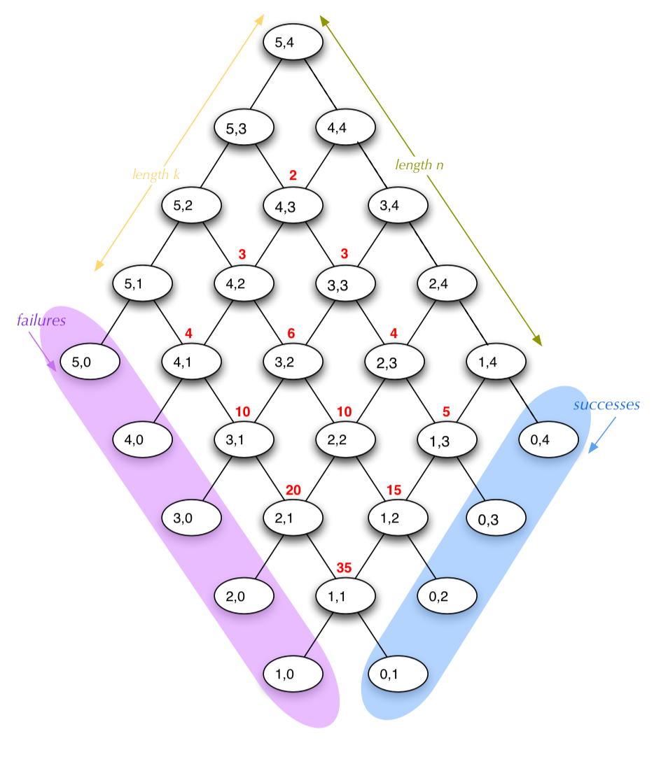
Since the number of times each interior node is called is the sum of the two nodes above it, and the top edges are all 1, what we have in the middle is a portion of Pascal’s Triangle. We can use the properties of Pascal’s Triangle to help figure out how many procedure calls in total there are.
For one, any entry in Pascal’s Triangle can be calculated from the row and offset into the row using the choose function again: it is simply C(row, offset). Another property, very useful for us, is what’s called the ‘Hockey Stick Rule’, due to the shape it describes. If you wish to know the sum of any diagonal of numbers extending from the edge to somewhere in the middle of the Triangle, it is the number just below and in the opposite direction of the diagonal. Expressed using the binomial coefficients (i.e. the choose function expressions), the result is:
| m-1 | C(r+i,i) = C(r+m,m-1) |
| Σ | |
| i=0 |
In that expression, r is the row the diagonal starts on, and m is its length. Note that we start our row and offset indexing at 0 when using these formulas.
We’ll split the total calls into two types — those that terminate and return a single value, and those that do not immediately terminate and rely on the calls below them in the tree.
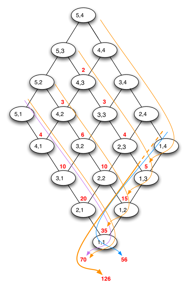
The calls that do not immediately terminate form the parallelogram-shaped portion of Pascal’s Triangle. By the Hockey Stick Rule, the number of calls made for each diagonal line sum to the value at the end of the line just below it (see the orange lines on the diagram below). This means that the total calls in a diagonal match a diagonal, or at least nearly one, made up of the values at the ends of the rows, plus one more value further into the interior. The outer value ‘1’ is missing in this diagonal. For the moment, we’ll ignore that and just consider the whole line. Using the Hockey Stick Rule again, it sums to the value just below and in the other direction from that diagonal. This leads to the entry straight down from the bottom tip of the parallelogram (two rows below it).
If we sum our diagonals along the n – length side of the parallelogram, the ‘summing’ diagonal starts on row n – 1 of the triangle. There will be k + 1 more rows, including the extra one to complete the diagonal, and the offset value will also be k. The formula for Pascal’s Triangle gives us the value for this sum as C(n + k, k). We can use the fact that for the choose function C(a, b) = C(a, a-b) and rewrite the result as C(n + k, n + k – k), or C(n + k, n) .
Next there are the terminating calls. The successes (i.e. valid change combinations) will come from calls at the lower right edge, and there will be just one for each call to its upper left. This just copies the bottom diagonal of the parallelogram. Similarly, all the calls that end on the lower left (failures) will occur once for each call on its upper right. The total number of terminating calls will be the value one below and to the left of the parallelogram (for failures), and one below and to the right of the parallelogram (for successes).
Those two values are in fact in the Triangle just above the sum we figured for non-terminating calls. That means the number of successes and the number of failures sum to that same number. A diagram of how these sums come about for the values already considered is shown below. The orange lines show totals for nonterminating cases, the purple show failures, and the blue show successes.
The total number of calls, then, is twice that number. Although we have to remember to subtract the 1 we ignored earlier.
Total procedure calls: 2 * C(n + k, n) – 1
As a quick check, we can also compute the total number of successes, which is the answer to our routine, using the Hockey Stick Rule. The starting row index for successes is n – 1, and there are k of them. The formula gives the result C(n + k – 1, k – 1) which is again equivalent to C(n + k – 1, n) . This matches the value as figured previously.
It’s important to remember that I have only shown this to be valid for this particular subset of the original procedure. I claim (without proof) that this is a “worst-case” class of the problem. Running this with unique positive integer values for currencies should take a number of steps that are some fraction of this value. Even if fractional coin values were possible, the values could be normalized without changing the amount of time taken. The claim, then, is that if this case is O(f) then all sets of coins will complete in O(f) time.
A simpler bound more useful for comparisons can be derived by breaking down the expression another way. This is derived from the definition of the choose function, and by reducing some of the terms in the factorial expression.
| C(n + k, n) = | ( n + k )! |
| n! k! |
| C(n + k, n) = | ( n + k ) * ( n + k – 1) * ( n + k – 2) * … * ( n + 1) |
| k! |
| −1 + 2 * | ( n + k ) * ( n + k – 1) * ( n + k – 3) * … * ( n + 1) |
| k ! |
The growth of this is determined by the fraction’s numerator, which will be a polynomial in n having n k as its highest term. The time taken increases at a rate no worse than n k. Written using Big-O notation, the time complexity for the procedure is O( n k).
I did write some routines to try and test this. It’s obviously impossible to empirically prove something true for all values, and it certainly doesn’t give the exact bound of the result. Instead, it serves as a sanity check on our result. If something wildly different from what was expected shows up, then something is wrong about the result (or the testing method, perhaps).
The test procedure makes use of the display routine which hasn’t been encountered in the book, although it will show up soon enough. It’s simply used to output something to the screen. newline, as might be expected, ends the output line. The test uses an altered version of cc, cc-counter, which performs almost the same calculation as cc but instead returns the total number of times it is called, by simply returning or adding 1 in all cases.
The critical part of the test procedure is determining the call count compared to n k. If the procedure were exactly on the order, then this ratio would be constant. As it is, we only expect O( n k), meaning that it should do no worse than this. And if it stays roughly in the range, then our calculation is a good estimate. My tests show that with the same value of k, the fraction does stay pretty close; at least in a narrow range and apparently decreasing with higher n, which is a good sign. Changing k also has the effect of reducing the ratio (as expected from the reduced fractional form above). This suggests that, for this version of the problem at least, the actual complexity could be a bit smaller, but still does not grow faster than nk. It should be noted that this remains only a measure of the number of calls, not the real time taken in the procedure.
Ex 1.15
There are a couple ways to determine the answer to this problem. One way is to work it by hand. Not too many steps are required, so it’s not too onerous. A better version of that is to use a debugger to step through the procedure. This does much of the same work, but with the advantage of no inadvertent mistakes that result in a wrong answer. The procedure is given to us, so we simply have to follow it.
I’ve done the ‘debugging’ in a crude way, making use of the display procedure to show the answer. Each time p is called, it prints out a line. Counting those lines gives the answer. Normally this isn’t a great way to accomplish this task (for one, it changes the routine as given to us so is in a sense incorrect; our p is not the original p but common sense says the number of calls is the same). This method is easier to repeat in a file, though, and takes less time. There do exist debugging tools that would count the calls to a procedure without requiring you to rewrite it. That would probably be the best way to handle it if doing this computationally, quickly, and repeatably is desired, although some time must be invested learning to use them for your implementation.
The second part of the problem in this case is much simpler than in 1.14. For one, this is a straightforward recursion, with the number of calls to sine being the primary factor in both the space and time required. Both of them can be found by figuring the number of calls needed.
Repeatedly dividing by 3 means that we are expecting the value for angle a to be 0.1*3x, with x an unknown value. To make this a little more generic, let’s replace the value 0.1 with ε, the understanding being that it is a nonzero positive value small enough to allow for termination. It should be clear that ceiling(x) (the closest integer >= x) is the number of divisions required before the value is less than ε. We need to figure out what x is, then.
a = ε * 3x
log3a = log3(ε * 3x)
log3a = log3ε + log3 3x
log3a – log3ε = x
log3 (a/ ε) = x
The ceiling of this result gives us the order in time and space required.
To check this (and as yet another way to solve part a), we can answer the first question asked using the numbers given. To figure the calls required for sin(12.15) with ε = 0.1, we have log3(12.15/0.1) = 4.369; the next integer is 5, which is the right answer.
Since ε is a fixed value and not a variable, it will not affect a practical consideration of the order of growth to ignore it. Similarly, if we only concern ourselves with orders, the base of the logarithm makes no difference either. In this case we can simply express the time and space as being O(log a) .