Part of the impetus for finally completing the previous post on how the site was built was that I recently made a number of changes to modernize the site. While the design remains mostly unchanged, it was at long last necessary to make a few improvements. I mainly wanted to make it more accessible for reading on smaller-size screens (like a phone), but cleaning up a bit to take advantage of advances in design languages like CSS was also a part of it. Fortunately those two went hand in hand, since naturally many of the developments in CSS were meant to make adaptive designs easier to manage.
The previous design had a rather straightforward, somewhat strict design approach. Since almost all of the site’s content is in the posts, I decided on a fixed ‘optimal’ page size for a post, and everything was measured out according to those rules. It made it easy for me to deal with the CSS. If I needed to size an element, I could choose the exact pixel height and width. About the only concession was that I tried to handle font size adjustments a bit better, since I often resize text depending on my viewing device. That’s not to say I did it well, just that I didn’t really attempt to make any other adjustments.
Of course such a site had the advantage that it always would stay the same, no matter what device you viewed it with. I didn’t need to worry about elements appearing in wrong places or being squished or distorted. However, that also meant that anyone trying to read it would have to keep scrolling around the page. It would end up appearing like a snapshot of a page in a book, or a newspaper, or a PDF file, with only a tiny window into it if you had a smaller screen. There were probably portions of it that were almost hard to find at times, and it was possible to scroll over to a largely blank section in places.
To replace it, I wanted something that would make it possible to preserve the traditional view, without necessarily forcing it as the only ‘correct’ way to view the site. It turned out to be not all that difficult. I chose to define a ‘smaller’ size at about half the previous size’s view, with a larger size that would be more adaptable from the fixed width of the older design. Setting that up was done using a CSS grid layout. It’s a fairly simple one, since I don’t have very many page elements. That required some adjustment as well to the pages that weren’t just an article (in particular, the topic sections), but moving away from the fixed pixel sizes made it possible to clean up the layout a bit. It also allowed for the page to work well when expanded to even larger sizes, which I found to be a nice bonus.
The ‘smaller’ size naturally required the most re-designing, since some elements had to be repositioned without disrupting the general style I want. It did introduce a few design bugs, and some things that I’m still noticing. I can no longer expect the design to always look the same on all devices, and especially not on all browsers. That may never really have been the case, anyway, and hopefully it is all still usable on any device, but now easier to use on smaller ones.
At the same time as I was updating the layout, I realized it would be a good time to also update something I had wanted to update for a while, namely the photo galleries. The photo galleries were always a minor part of the site, and fairly small, but I still would like them to be functional. They are the one part of the site where I don’t mind using a different design style, and also have the only significant amount of Javascript (so that a gallery can be browsed more conveniently). Previously I had used Rhotoalbum, which is essentially a script that did static generation of a gallery from a folder of images. It was okay, but not something I particularly loved. The piece of Javascript it depended on previously (and loaded remotely) had also finally gone away, and while there was a version that included it directly, it was a suggestion to me that I should try something new.
I still wanted something that could run without having to tweak too much, and generate galleries in much the same way Rhotoalbum did. However, there don’t seem to be that many projects that do quite what I wanted. I tried several, and they were either non-functional, or required more configuration of the images, or configuration on their own in order to work. The farthest I got was with Sigal, a static generator written in Python. However, I found that trying to customize it to the way I actually wanted to lay out the gallery did not quite work, the biggest issue being trying to skip over certain directories in the image folders. It had already been a struggle to get it even working properly, possibly due to Python versions (or dependencies), and since I’m fairly unfamiliar with using Python, it was becoming an uphill battle.
However, I did like one of the galleries that Sigal has as an option, namely Photoswipe. It occurred to me that the side of Sigal that I was wrestling with — configuring the images and loading them into a gallery format — was something that it would not be too hard to script on my own. It was the controls and interface of the gallery that I didn’t know how to do, but since Photoswipe appeared to be a distinct project, it seemed like I could find some way to incorporate it on my own pages. Not to mention that I already was using something that could generate static pages — Jekyll.
I abandoned the attempts to use static gallery generators, and relied on Jekyll instead, with a custom script to bridge the gap of making an index of image files. I used a Jekyll collection with a bit of custom front matter. This has the distinct advantage of allowing me to structure the gallery entirely how I want, as the Jekyll collection does not have to match the file structure (or the directory names, another issue I was having). The only restriction is that each gallery references a single directory of images, although technically I could probably work around even that. The custom script runs through the image folders and generates a YAML index file that provides all the image information that Jekyll and Photoswipe need (image size and location); it will generate thumbnails as necessary, and it will also try to preserve any existing index files.
That does make it slightly more work than any of the gallery generators, but not by much. Adding a new gallery means adding a new file to the Jekyll collection (I have a ‘galleries’ folder), which includes the source directory, the gallery description, and where the gallery should appear in the hierarchy of the site. The way it is set up, my galleries can have photos of their own as well as sub-galleries, and each sub-gallery has a parent that it can link back to (the ‘to upper gallery’ link at the top of the page). About the only disadvantage is that the gallery description is not located with the folder of images, but that could even be seen as a feature if I want to reconfigure the gallery for some reason. The index of photos stays with the folder, since that makes more sense as the image details will stay with the image, regardless of the gallery they end up in. This index file is also where I can add alt text/titles to the photos as needed, which is another feature I wanted to make relatively painless.
Once I had the Jekyll collection generation set up, it took only a little more work to get Photoswipe running properly. This was mostly down to working out a few details with the options. The biggest headache was with gallery names, as certain things would not be processed properly, such as spaces in names. As a result, I simply needed to use a distinct ‘gallery name’ that Photoswipe could use if the original directory could not be used. It appears that it is all working correctly now, and as an added bonus the gallery pages are styled more in the way the rest of the site is, instead of being distinctively different as they were when I used Rhotoalbum’s defaults.
All of these changes are relatively new, and I haven’t really had a chance to test what it will be like to modify the photo galleries yet. That will indeed be the way to see if what I’ve done was a good idea or no better than before. I am, however, hoping for the best.
Website
Building the site (part 2)
November 14, 2022 11:29
Part 2: Textpattern and Setting up the Site
Well, I did say there’d be a next time… and here it is just a decade later. In the intervening time a fair amount of what I went over in Part 1 has been rendered obsolete. On the other hand, what I had so long ago intended for this post to be about is mostly the same (since it’s partly about what I did). Indeed the process I use has hardly changed either. I now likely have a topic for another ‘site-building’ post, detailing some the recent changes to modernize the layout a tiny bit, and to change the photo gallery so I can put up some more photo sets.
Briefly, I’ll go over what is no longer relevant from the first part. As already mentioned there, I switched from using categories as post labels to tags, since they seem more flexible. That’s still how I mark the posts. For the topic index page, I was able to ditch my custom page_lookup Liquid tag by switching to Jekyll’s Collections. A Collection in Jekyll is basically a set of related content that has documents stored in one directory. Previously I was storing all of my ‘topic’ descriptions in one directory as well, so it was hardly any trouble to just move them to the _collections directory, and then adjust Jekyll’s config file to produce actual pages for the collection. Jekyll then automatically makes the YAML front matter from the collection files available when iterating through a collection item.
Now, for what this post was ostensibly about, the migration from Textpattern. Jekyll has migrators available for a fair number of blog engines, although I’m not sure how many of those engines are still in use. (sidenote) Textpattern CMS is still going strong apparently It would seem that simply running the Textpattern importer was all that was needed. The importer indeed worked fine, but it only pulled out the content of the posts themselves. I also had several photos that were associated with the posts, and the image tags wouldn’t get processed. The slightly tricky part, which made it more than a matter of just replacing the tags, was that Textpattern had multiple types of tags. I had regular image tags, ‘article’ image tags, and also ‘thumbnail’ variations; additionally, images could be indicated by either name or database id. At the time, I modified the Textpattern migrator to also process the image tags and simply turn them into HTML image tags in the imported articles. I also copied only the image files that were needed to a new directory. It may be that the importer now handles images this without any issues; I haven’t really checked up on it.
One legacy of using Textpattern is that all my posts were formatted using Textile. In the course of time, Markdown has seemingly won out almost everywhere, and Jekyll itself expects Markdown to be used (although the Textile Converter plug-in is available.) I still use Textile, using that converter. While I do prefer Markdown’s link syntax and a handful of features, the one thing that it’s missing that Textile supports is easy use of italic tags alongside em. Markdown avoided ‘confusion’ over the use of * and _ by making them identical, with doubling being the distinguishing feature, to handle em and strongHTML tags respectively. In Textile these symbols are sensibly distinct, and the doubled version is used to indicate whether italic should be used instead of em, making it easier to have both in your text. If you are wondering why I want that, it’s because I’m often using algebraic variables or terms that should be using italic. In truth, I rarely use em, but it is good to have an easy way to use both.
Something that I did give up when switching from Textpattern was the ability to create and edit posts directly via the site itself. When I was traveling and had very limited internet access, that was invaluable. Jekyll doesn’t do that on its own, since it does not ‘run’ while the site is active, it just generates the pages. That’s more of an advantage for me now, since I use Nearly Free Speech to host the site, and it’s very inexpensive if the site is static with no databases. Now technically, since Jekyll could process the pages and make a new site quickly, I could set things up to just use a text editor, put the file on the site, and regenerate it on-the-fly. In practice, since I use my laptop to write the posts now anyway, I don’t really have a need for that. In fact, I don’t even run Jekyll on the site’s server.
Initially I did edit files on my side, uploaded them, and then ran Jekyll to build it on the site. However, I wanted something that didn’t require as much interaction, since at the time I would have to log in and build it manually. I could have set up a script that would trigger when the files were uploaded and then build the site. The problem was, what happened when there was an error and the site was not rebuilt? I needed to not just be sure that the file was uploaded, but also get feedback on the Jekyll error, and then run through the process again until it worked correctly.
It was tedious to edit, upload, and then have to check to see if there were any errors reported from the generation process. And as often as not I also wanted to test the site locally before making some change, to see how it looked before making it live. While a more complicated script (or some other system on top of Jekyll) might handle that, I wanted it to remain simple. In the end, it was easier to generate the entire site locally, and only upload the final product. I use git to keep them in sync, and to ensure a stable version if I need to revert some changes (just in case, though I’ve never had to actually use this capability). It lets me do all the editing and testing on my own machine at my leisure, and also limit server usage to only keeping the files of the actual site itself. In theory, it would also work just as well if I stopped using Jekyll, as long as whatever I used created a complete site.
While it might also reduce the files stored on the server, in practice I do something that effectively keeps a second copy of the whole site. The git directory I upload to is not the one the server uses as the site (in NFSN, the ‘public’ directory). Instead, I have a post-commit hook script that copies all the files out of the repository. Here’s the heart of it:
It first uses git to create an archive (a copy that doesn’t include the repository history) and outputs that to a temporary directory. Then rsync is used to copy the files to the public site (i.e. directory). The first set of options to rsync there are -rlt to copy recursively, include links, and copy file modification times. The -vi options output an itemized list of changes for monitoring the process during the upload, and the delete option removes the files on the server that are not in the current repository. Afterward, the temporary copy of the git repository is removed. Using this method, the public site never has any files but the latest version from the repository, and none of the git history. The rsync copy step might not be strictly necessary, though it gives me a little bit of peace of mind about some file copying errors. There’s maybe also a reduction of the brief time window during which files on the server might be changing, but given the static nature of the site, and relatively fast internet connections, that doesn’t amount to much of an issue these days.
As mentioned, there probably is enough for me to do another post on the recent updates, most particularly the changes to the photo gallery. I make no promises about when to post it, but I expect it to appear in less then ten years.
SICP
SICP 3.5.5
July 25, 2021 11:36
Exercise 3.81
The basic form of the solution is to take the rand procedure that accepts an argument, and use stream-map to apply it to the input stream. Minor adjustments need to be made so that the requests are accepted in the format used by the stream. To make a version that does not produce output on reset requests, just add a stream-filter using number? and have the internal resetting procedure return a non-numeric value.
There is one more consideration for the stream version. To prevent two such random stream generators from interfering (in the manner of the ‘concurrency’ test), each needs its own pseudo-random number generator. If there is only one global PRNG, then the sequence will be inconsistent when requests are being handled by two different stream processors. In Racket, a new PRNG can be created using make-pseudo-random-generator, and passing the generator as an argument to the random procedure. The reset takes a little extra effort (as only the ‘current’ PRNG can be reset). In a truly concurrent system this reset would need to be handled using a synchronization mechanism to avoid problems. Other interpreters may have their own means of making new random generators. Alternatively, the PRNG can be a procedure of its own and avoid using the system’s built-in random number methods. (see 3.1.2, when the original rand was discussed, for more details).
Exercise 3.82
In order to model this after the version from Exercise 3.5, it’s useful to define random-in-range to work on a stream. Naturally the stream of random input values is one generated using the solution for Exercise 3.81; I used constant-gen as the request stream to just keep producing random values. Since this version of monte-carlo needs an experiment stream, not just the experiment as a procedure, we have to define a recursive stream-generation function that computes success or failure, and takes a random stream as its input (this is an internal definition, so P is the predicate already passed as an argument).
(define(experiment-streamrand-stream)(cons-stream(P(random-in-rangex1x2rand-stream)(random-in-rangey1y2(stream-cdrrand-stream)))(experiment-stream(stream-cdr(stream-cdrrand-stream))); taking two values at a time))
We have to take two random values at a time from the random-stream, which is why this can’t simply be another stream-map. It could be possible to use mapping by using multiple functions, but it’s reasonably easy to handle it in this fashion. This procedure does assume the random stream will be infinite, and therefore does not check if it can take two more values or not. This is an optimization to speed up the processing, since it really should not be run with a finite stream.
The last step is to compute the total area in order to scale the results properly. That leads to a call to scale-stream around the call to the stream version of monte-carlo. The inputs are set up with the initial values of passes and failures set to 0, and that is our final stream.
This is a brief section that continues the theme of practical uses for streams. This time there isn’t anything particularly intricate related to internal workings of the stream. Instead, it’s leading toward a particular idea, of a stream that can create the same effect as assignment to change state over time. Far from being an esoteric side topic on the way to building programs, it’s an idea that has garnered some interest in recent years, as it is at the heart of something called Functional Reactive Programming. If you’re interested in knowing more, you can search up resources on that topic.
There are only two exercises in this section. Because the results are partly determined by random values, it’s not possible to do a completely reliable test of all the results. In the first exercise, we can at least check that the output is repeatable, as that is a requirement. The actual values still need to be observed, though; a faulty implementation could produce output that passes a ‘repeatability’ test fairly easily. The randomness also means that we can’t guarantee a test did not pass merely by coincidence, nor can we test reliably for a negative outcome (i.e. test for patterns that ‘should’ be different). There are some statistical approaches that could be used if we actually wanted to test such a system, but I feel that would be taking the topic a bit far afield. This isn’t about random numbers, it’s about stream processing.
The text also doesn’t completely specify how the stream of requests is formatted. I made it so that the elements of the stream are either the token 'generate, or a list in the form ('reset x) where x indicates the number. The reason for using a list instead of a simple pair is so that input streams can be written out more straightforwardly as quoted lists. To simplify the creation of the input even more, there’s a procedure that converts ‘abbreviated’ forms (using the letters g and r instead of the full words). To use the test input streams, make sure that your version accepts requests in the full-word form. Additionally, the wording of the exercise seems to imply that a reset request might also give an output of the specified value, as it refers to resetting the ‘sequence’, whereas generate makes a ‘new’ value. Some of the tests that rely on stream references have an alternate version, depending on whether resets produce output or not.
One of the test sequences also checks that two streams produced in this fashion do not interfere with each other when they are run ‘concurrently’. This isn’t so much concurrency from a processing point of view, but in terms of the event streams. We know (or can expect) that the random values in the stream are not actually computed until the first time an element of the stream is referenced. We want to ensure two things: Firstly, if we access the same stream reference later on, we don’t get a different value. (This is likely handled by memoization of streams). Secondly, we need to make sure nothing disrupts the way the random numbers of a given stream are generated, so that ‘the same’ calculations produce the same result no matter where they occur in stream time or actual time. Technically all that is needed in this case is that a reset command produces the same output sequence after it, and we can’t be certain of ‘when’ the calculations occur (e.g. what we call a stream might pre-compute 5 or 10 random values in advance, and we’d be none the wiser). So it’s still a bit questionable from a testing point of view. If this part is giving you trouble, consider it optional, but at least be aware of it as something to keep in mind if taking this section’s functional approach to time-ordered events.
The second exercise is to redo Exercise 3.6 using streams. While there are definitely some functions from that exercise that would be useful to include here, I consider it an element of the exercise to understand just what can be re-used and what might need to be updated. I did, however, include an implementation of a Pseudo-random Number Generator, and a few interface functions for it. You may choose to use this one, or whatever built-in random function your own interpreter uses.
A straightforward way to solve this one is to just wrap the old version of the integrator with a let statement that forces the delayed integrand. There may be alternate approaches, but since we already have a version that works with a non-delayed argument, it may as well be re-used. That said, it’s not sufficient to drop it in as-is, since the procedure is recursive (for this reason we can’t simply call the old procedure). As we know from the previous exercises, recursion within an argument expansion can cause problems when streams are infinite. It must be changed to include a delay statement on the argument being passed.
Exercise 3.78
Each of the blocks in the diagram can be interpreted as a function, with the labels naming the streams used as input or the output of those functions. That allows the solver to be created quite similarly to the way the first solve function was created.
The implementation here is nearly identical to the specialized case. The only difference is that instead of the stream ddy being fully defined in advance, it will be formed by using the function passed as an argument, with a stream-map. It actually ends up being shorter, thanks to the power of stream-map with arbitrary arguments. The streams y and dy are the ones mapped to the function f. That allows any function of two arguments to be used, and the solver’s output will be a stream.
Exercise 3.80
As in the RC circuit, the functional blocks outline the structure; each can made into an internally defined procedure that generates the labeled streams for the block. The complication here is that the initial values are not known at the time the RLC procedure is run. If we defined the function block streams within RLC, we’d have to include some way to pass the initial values and generate the streams from them, possibly by passing the initial values along in the streams, or by having a ‘manager’/interface function that sets them as internal variables. My approach wraps all the block definitions inside the function that is returned. This way, they become internal not to RLC but to the stream-generating function that it returns. Producing the procedure’s output is not difficult either, as all that is needed once the internal streams are defined is the cons statement at the end to give the desired result.
We are still looking at infinite streams. The last section covered a lot of ground in the use of infinite streams, whereas this one focuses in on one particular aspect. Namely, the delayed evaluation that is critical in allowing streams to be effectively infinite, without causing programs to end up in an infinite loop when processing them. In some ways this section is just an expansion on the problem encountered in Exercise 3.68, in which the lack of a required delay led precisely to the infinite loop problem.
The exercises in this section deal more with the applications of streams than the abstractions of creating them. They also get heavily into numerical methods for solving difficult math problems. This not only poses a problem if you don’t have much of a background in engineering or higher math, but it’s inherently hard to really test the exercises for exact results. Even coming up with good test cases is difficult. These types of problems aren’t always the sort with intuitive or simple expected results that can be understood by just looking at them. There are additional pitfalls that come about not because of the programming problems but simply from the methods being applied. So, despite the relatively few number of exercises and programming work to be done, actually verifying the solution requires additional work and knowledge.
These application-oriented exercises can be of interest to show how much can be done with an apparently simple program. I think at least partly that seems to be the authors’ intent. (Arguably it was much more impressive when computation of this sort was a bit rarer). The types of calculations are at a high level, and it shows just how powerful recurring/infinite streams can be when used the right way. I’ve tried to choose examples with more easily-understood results that still show off some complex behavior. If you’re not interested or you lack knowledge of these topics, hopefully you’ll still be able to figure out from the examples whether the system is working as expected.
This is a set of exercises where testing the results by checking against a few (or even a list) of pre-determined results won’t cut it. Perhaps that could be done in some cases, but I’ve left it fully open to interpretation and observation, since some understanding of what the expected results even look like is necessary. In some cases the results should not even exactly match the ‘expected’ ones, but just approximate them, with some of the input variables allowing for refinement of the output. This post will be a fair bit longer than others on the exercises, and go more in depth on the test cases, since I’ll be giving an explanation of what each system being tested should look like, in case you are unfamiliar with the underlying topics.
First off, there are just a few new functions, and they are all included at the top of the exercise file. (The file with additional stream functions, used in 3.5.3, is still required, though.) One that will be useful for analyzing mathematical results is the generate-check-list, which will produce a list of stream indexes to check, based on a given ‘step size’, a common element of these solvers. Instead of having to look up what the 500th element of the stream is, this will find the value the stream has for a given value of the input variable (e.g. x or t), regardless of step size. Given a list of input values, it will give the output generated for those values, wherever they show up in the stream. That allows us to vary the step size and still compare results directly. Another function that may come in handy (and is already in the included files) is stream-reduce, a function I wrote that filters out most values in the stream, producing a reduced stream of every nth value. That lets us observe changes in the stream values more readily than if we had to examine a long list of numbers that are only slowly changing when the step size is small.
In addition to using functions like stream-reduce, it’s probably a good idea to use a graphical tool to plot some of these number lists to see if the results fit expectations. Since the last section, I discovered that in Racket at least, there is a built-in plot function that makes simple charts in-line (there are some usage examples at the end of the exercise file, for Exercise 3.79). It’s possible that your Scheme interpreters may have something similar, or you can copy out the resulting numbers and plot them with other software.
Obviously, unless you know what to expect from these mathematical functions, even visual plots are not meaningful, so I’ll briefly go over the examples I used for each exercise. Of note if you’re totally unfamiliar with the topic, I may use an alternate notation for derivatives as follows: If our function is y(t), y′ indicates the first derivative with respect to time (also called dy / dt), and y″ means the second derivative. It’s easier to type and is fairly common as well. Furthermore, the ‘initial value’ provided to the solver is what y(0) is (along with y′ (0) in the second-order solver), so those terms can be used interchangeably.
For the integrals and the initial solver, the book has only the simple example of dy / dt = y ( which could be written y′ = y ). This is solved by functions of the form et + C ( C is a constant we can choose by setting the initial value). That yields the number e when t = 1 and the constant C is 0, which lets us do a simple check if it does produce that value when evaluated. For another example of straight integration I used a polynomial, which will have a polynomial answer (of one higher degree than the integrated function); an initial value of 0 is easy to use there as well, and the polynomial calculation can be done directly to compare the results.
For a more complicated differential equation, I used y′ = 3 y2 + 2y + 1. This has an exact solution of 1/3 ( sqrt 2 [ tan ( (sqrt 2) t + C )] – 1, where C again is a constant we can select. I chose C so that an initial value of 1.0 can be used. There is an obvious problem with this solution, however — it is only valid for the points at which the tangent function is defined. This was done deliberately and demonstrates what happens when the numerical methods have to be compared to asymptotic limits of the solutions. It becomes tough for a computer to properly calculate results with our solution, even when we can state it exactly as a function. It even becomes hard to say which value should be considered more inaccurate, as we’re going to be depending on Scheme’s own mathematical functions (which internally is also going to depend on numerical methods). We can look at behavior over the whole range to see if it matches, but we do need to know over just what range we can expect to compare our answers. See the exercise file for more details.
The second-order solvers of the later exercises build up from a simpler case to a more general one. The initial solver deals with homogeneous linear equations only. These can have an easy solution of ert if a and b are properly chosen; the value of r is found by simply solving a quadratic. That works well to test this case, since the solution’s values can be checked quickly. That equation can also be tested with the generalized solver.
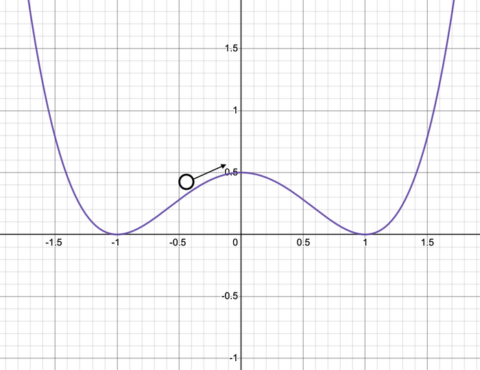
Of course, we would also want to check a non-linear equation with the generalized solver, too. That is starting to hit the limits of what is easy to test our answers against, and for many people (including myself) the limits of their mathematical knowledge. I chose something called the Duffing equation, which can model a variety of physical phenomena involving oscillatory behavior. The form I used has a y3 term and a term with y′ (the first derivative of y) in it, along with a ‘damping factor’ signified by gamma (γ). This models an object that could end in a ‘double well’ — imagine a ball rolling in a container that has two resting points and a hump between them, with infinitely high walls on either side hemming it in. The variable y represents position relative to the origin (where the central hump is aligned), and y′ is the ball’s velocity. Bear in mind this only models one-dimensional motion, so the ‘ball’ would be sliding back and forth. Then, the ‘wells’ will be at +1 and -1. The damping factor represents the loss of energy (and thus speed) over time, which could be friction against the surface in this example. Here’s a graph to illustrate, but remember that y in the equation represents the horizontal position (distance left or right of the origin); the vertical position is not modeled.
After some amount of time, the ball will come to rest in one of the wells. Which one it is depends a lot on the initial conditions (where it starts and how fast it’s moving) and the damping factor. It’s hard to really measure how accurately the solver is doing with the specific values, but the trend to settle on one side or the other should be plain during testing. The solver is likely either working correctly and approaching one of the two long-term results at +1 or -1, or not really working at all and giving impossible results as time goes on. (Note that altering the timestep may drastically alter the values; this is a very sensitive system.)
Finally, there is the RLC circuit, which is a practical example of a system modeled by differential equations. The signal-flow block model is hopefully sufficient to show how to create the solver if you don’t follow how the circuit works. Here, we can generate a test case using the original values from the text, but we need to know what to expect as output. It turns out there are a few interesting cases to consider, including one that showcases another potential pitfall of numerical methods (not really a problem with streams).
Firstly, here’s a brief explanation of how an RLC circuit works. There are two elements in it that store electrical energy (as charge). The energy stored on a capacitor (the ‘C’) can be measured from its voltage, and on the inductor (the ‘L’) it is a function of its current. These two elements don’t produce any energy on their own, but they don’t consume it either These are ‘ideal’ circuit elements, analagous to frictionless surfaces. If either component has some initial value of voltage or current, the charge will transfer back and forth between them. The voltage on the capacitor will turn into current in the inductor, and vice versa. With just these two components (an ‘LC’ circuit), the oscillation would continue forever. However, the third element of this circuit, which is the resistor R, does nothing but dissipate any energy that passes through it. So when the resistor is part of the circuit, the energy that flows back and forth between the inductor and capacitor decreases a bit at a time until it is totally dissipated by the resistor (as heat).
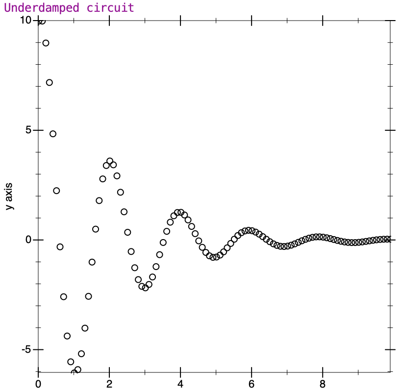
The values given in the example demonstrate the fading oscillation fairly well; the values for both voltage and current go up and down, and decrease in amplitude with each cycle. Here’s what the plot looks like from my runs in Racket.
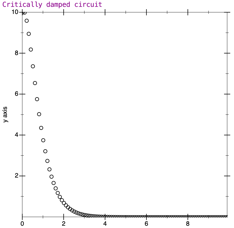
The actual time taken for each ‘cycle’ (from one peak to the next) is determined by the L and C values, and the rate of decrease is determined by the resistor. What happens when the resistor is large enough that the energy is dissipated before the oscillation even starts? Similarly to the Duffing equation, we can define a damping factor (traditionally for this equation zeta [𝜁] is used, not gamma). The damping factor indicates how much relative oscillation will occur. In the situation where 𝜁 = 1, the system is said to be critically damped, and is right at the point where the energy fades just as oscillation is about to start. Here’s the plot of a critically damped system with characteristics similar to the original example.
When the damping factor is lower, we would say the system is underdamped, and some oscillation will always occur. This is the case for the text’s example. If 𝜁 is greater than one, the system is said to be overdamped, and will not oscillate. What is interesting in the overdamped system is that while it goes smoothly toward zero without oscillating (the curve resembles the critically damped case), it takes longer to do so than in the critical case. Circuit designers would need to balance the response time of the system with how much oscillation is acceptable, and choose the damping factor appropriately.
This may have seemed like an unnecessary digression on the workings of this circuit, but I wanted to highlight something about this model. There’s a problem that can arise when we simulate an overdamped case. If the overdamping is very high, and we otherwise use the same simulation parameters from the other cases, we may find that the numbers start to increase without bound. This is not something in the mathematical circuit model per se, or an error with the stream paradigm. The problem is that the timestep might not be appropriate to simulate the changes in the system. In this case, we have to reduce the size of the time step to get correct results.
It is somewhat counterintuitive that the ‘slower’ overdamped system, which doesn’t display a change as rapidly as the others, can have this issue. An issue at the other end of the scale, where a fast oscillation is skipped over when the time step is too large, might be expected (and certainly could happen). Yet, as this demonstrates, problems with numerical methods can creep in regardless of what the scale of the system might seem to be. There are truly a host of issues that are well beyond the scope of this exercise. It’s just worthwhile to know that not all problems are due to faulty procedure implementations.
In the original version of sqrt-stream, a single stream is defined. It then maps onto the exact same stream, which is named guesses. In Louis’s version the stream is mapped to a call to the procedure sqrt-stream which constructs a stream and returns it. That means that an entirely new stream is constructed with each ‘recursive’ call. One advantage that the original has is that the same stream is being re-used in the mapping, possibly representing a savings in space when computing new values. More importantly, each time a new element of the square root stream is generated, the original version will have already calculated and stored the previous guesses (assuming memoization is used). With Louis’s procedure, all elements of each new stream have to be computed every time. The number of steps to calculate the nth element is the sum of integers up to n; this is O(n2). The original version, meanwhile, is O(n) with respect to calculation, since each value is computed only once and then memoized for later access.
There is still some memoization that occurs in Louis’s version at the higher level. If the result of the sqrt-stream call is itself defined as a stream, then future calls to already-computed values will be memoized and no additional calculations are required. Only if a call is made to a higher number of elements later in the stream will the extra computation result. There is no difference at this level between the two streams as both will benefit from memoization in this way. This is demonstrated in the testing by repeating the call on the stream; in both versions the second call will return without needing to call sqrt-improve.
The exercise also asks if there would be a difference if we were not memoizing calls to delay (at least that’s how I’m interpreting this; see the last section for the ambiguity on special forms for delay). I’ve already alluded to the idea that in the original, with guesses defined only once, there might be a space savings since it stays as one stream. Exactly whether this actually saves space relative to the repeated calls to sqrt-stream in Louis’s version would depend on stream-map. As it happens, stream-map creates new streams, and every new stream created is a computed initial value and a promise for the cdr, which means both versions are a single pair. However, Louis’s version will have one extra nested call, since it will have to take the stream-cdr of a new call to sqrt-stream at each step. The overhead of making a function call might be significant, but probably not compared to the computation of the value itself, which will likely dominate the extra time that Louis’s version requires.
Below is a diagram showing what is produced for each version when the stream’s cdr is taken (as in calls to stream-ref). I’ve simplified the expression a bit to just use ‘improve’ to label the internal lambda, and indexed the iterative guesses using the variable xi for each successive improvement. Note that while Louis’s appears to take up more space, it does not retain any references to previous elements of the stream, meaning that the previously created streams like ss1 can be deleted by the interpreter. In the original version, those streams (labeled g1, g2, etc.) need to be preserved, as the later elements of the stream refer back to them.
This procedure needs to take one value and then compare it to the next value in the stream. It thus needs to store one value from the stream and then get the next value of the stream to determine if the two elements are within the specified tolerance. The way I solved it is by using a procedure that takes a single value and a stream. It will compare that value to the car of the stream and return the stream’s car if they are in tolerance. If not, a recursive call is made using the car that was just read as the value and the cdr of the stream as the stream to compare it to.
Exercise 3.65
To express the formula as a stream we can follow the example of pi-summands and just use the next index as the argument (so that we use all whole numbers). Another approach would be to map the integers stream using division and flipping the sign when the integer is even. Either way, we use partial-sums to create the successive approximations. The accelerated streams then apply the appropriate stream transformation to the original partial sum stream.
Examining the first few results, we find that in ten iterations the original partial sum stream is still almost 0.5 away from the correct answer. Using Euler acceleration converges close to 0.69 by the second term and to the third decimal place within a few more terms. Tableau acceleration takes an extra term to ‘get started’ but within ten terms is accurate to more than ten decimal places. On many systems this quickly turns into an issue of precision, as in fact the sequence cannot compute any more valid terms as the floating-point math can no longer work with differences that are so small. That is an issue with the original pi-summands approach as well; creating a system that would operate to infinite precision is feasible but well beyond the scope of this section.
We can compare the number of terms required for a given tolerance to see just how quickly (or slowly) the three approaches arrive to the same precision. Getting to just three decimal places requires 1000 terms for the bare partial sums but only a handful for the accelerated sequences. We can compare the accelerated forms by looking at how quickly they converge to six decimal places and see that the Euler acceleration takes around 60 terms to just 5 for Tableau. The unaccelerated form would take prohibitively long to calculate with that precision.
Exercise 3.66
In spite of what the text implies about ‘qualitative’ statements, the thing I find easier to do is just examine the sequence of output and determine the mathematical pattern it represents. From there, I can work backwards to try and find what the underlying explanation for such a pattern might be. Here’s what we can observe from where certain pairs show up in the sequence:
(1 j) for j = 1 is at 0
for j > 1 will be at (2j – 3)
(2 j) for j = 2 is at 2
for j > 2 has a period of 4 starting at 4 (2 after (2 2))
(3 j) for j = 3 is at 6
for j > 3 has a period of 8 starting at 10 (4 after (3 3))
(4 j) for j = 4 is at 14
for j > 4 has a period of 16 starting at 22 (8 after (4 4))
(5 j) for j = 5 is at 30
for j > 5 has a period of 32 starting at 46 (16 after (5 5))
Finding where the pair (1 j) occurs is not too difficult to figure out intuitively. The first time pairs is called it will start interleaving with the stream created from pairing a 1 with all elements of the second stream. That means after the first output of (1 1) followed by (1 2), every alternate member of the output will be one of these pairs. Figuring out where (1 100) is as simple as multiplying by 2 (and subtracting 3 for the initial offset).
To get a more general formula, we need to find a pattern for values of i other than 1. The first time a new value for i shows up it will be in the pair where i = j. The next occurrence with that value i comes at some later point, but from then on it will recur at a fixed interval that is not the same as it took between the first two. The reason for this difference is that the first time, the new pair is coming from the interleaving picking the ‘second’ stream (where both i and j are advancing), and later on the pairs come from the ‘first’ stream (which keeps i the same and advances only j).
Both the first appearance of the pair including i and the first appearance of the next pair with i (where j = i + 1) follow a pattern based on powers of 2, since as we observe it takes somewhere near twice as long for each successive value of i to be introduced. In fact, the pattern for when i = j first comes up is just 2i, offset by 2. For the next pair that has i, we have to wait for one cycle of the next lower power of 2 (i.e. 2i-1) to finish. Thereafter we wait longer — the full value of 2i, and that does not change.
The result is that the index of a given term (ij) in which j > i follows an arithmetic sequence. The period at which it repeats is (2i), and that is multiplied by an index (j – i). It will have an initial value of 2i – 1 – 2. The resulting formula is thus:
The index of (ij) for j = i will be at 2i – 2
for j > i will be at 2i*(j – i) + 2i-1 – 2
If we apply the formulas to the suggested values we see that they produce very large values for even moderately low numbers. For instance (99,100) will be at 299 + 298 – 2 , which is position 950737950171172051122527404030, far too long to wait for the stream to produce! It’s more feasible to use smaller values to verify that this formula gives the correct result, which is why the testing numbers of 9 and 10 are used.
Exercise 3.67
In the original pairs procedure, the car of stream s was paired with every element of the cdr of stream t. Then this was interleaved with the result of pairing the cdrs of both streams. That ensures the car of t is only paired once (with the car of s) and then ignored. Using the stream of integers as the source for both, that avoids any pairs where the second element is smaller than the first. To produce every possible pair we just need to construct an additional stream that pairs the car of t with all elements from the cdr of s. We interleave this with the original streams to get the whole result. Then we feed it the stream of integers for both inputs.
Exercise 3.68
This exercise really gets at the heart of what often makes streams confusing to deal with. At first blush, it seems that this sort of operation ought to work with no issues. However, crucial to the processing of infinite streams is the ability to delay their computation until needed (also known as lazy evaluation). If this does not happen then it is all to easy for a stream processing procedure to get into what is essentially an infinite recursive loop.
What was missed here is that there is no delayed evaluation when constructing the stream in this version of pairs. Instead, it makes a procedure call to interleave. It may seem that this would not be an issue because internally interleave will call cons-stream thereby delaying the processing of the stream. However since interleave is a procedure, it must evaluate the arguments that are passed to it. What are the arguments passed to it? The first is a stream-map which will construct a stream and exit normally. The second, though, is a call to pairs. That’s where the trouble happens. Every subsequent call to pairs will again lead to an attempt to evaluate arguments to interleave which leads to a call to pairs, forming a recursive sequence that never ends, if either s or t is an infinite stream (and if they do terminate it will just be an error in stream-cdr).
It is therefore necessary to ensure that recursive calls in stream-processing procedures aren’t allowing this to happen. The recursion on a stream should only come inside a special form that won’t evaluate it as an argument — for instance using cons-stream, as in the original version of the pairs procedure.
Exercise 3.69
The construction of the triples can done in a way that resembles the pairs procedure. First, one triple is created from the cars of each stream. Next, we interleave the stream created by taking the car of the first, combined with the other two streams in a way that ensures the first element is smaller than the others. What we can combine with is simply pairs on the second two streams since that gives us exactly what we want (the second element is never smaller than the first). Finally, we call triples on the cdr of each stream, again using interleave to combine them. Of course cons-stream is used to build the whole thing, so we don’t end up with the infinite recursion witnessed in Exercise 3.68.
To generate a stream of Pythagorean triples we can construct a stream of all possible triples from the integers, and then use a filter to ensure they satisfy the formula.
The use of stream-filter allows for a fairly clear expression of the requirements on the output. We create a procedure that checks if the square of the third value is equal to the sum of the squares of the first two (since the triples are ordered by size, the last value in the triple must be the ‘longest’ side of any potential triangle). Notably, the production of the actual Pythagorean triples can be very slow, as the triples stream will have more and more invalid values the longer it goes on. While I did not calculate the actual index where Pythagorean triples are expected to occur, we can guess that similarly to the pairs procedure, even a moderately low set of values might occur at a very high index in the stream.
Exercise 3.70
At first glance it seems as though we could take the original merge procedure and instead of taking the leading elements and comparing them, just use the weights of the leading elements and compare them. However this probably produces unwanted behavior, because it seems as though we are now having merge do both sorting and combining. The problem with this approach is that the combination of the weights is distinct from the indexes. In basic merge, when the two elements are equal, only one of them should be added to the output stream. Elements with equal weight, however, might both belong in the output stream.
That actually simplifies the procedure, as we only need to consider which weight is lower when merging. Instead of a cond we can use an if statement. I also got rid of the let to get the car of the streams since the weights are only compared once. (The car of one stream is needed again when constructing the output, so it may be argued that it is worth keeping them as let-assigned variables, but more likely than not it makes little difference either way).
As for weighted-pairs, it almost exactly resembles the initial sketch of the pairs procedure in the text with the ‘combine-in-some-way’ procedure being merge-weighted, and an extra argument (the weighting function) added to its parameter list.
The stream in part (a) is constructed using weighted-pairs with the stream of integers as the arguments; the weighting function is just the sum of the two elements of the pair (note these are ‘pairs’ only using the terminology of the procedure; in actuality they are of list type and accessed as members of a list).
The second stream is a bit more complex to construct. We need to produce the stream of numbers that do not have 2, 3, or 5 as factors. This sounds like the inverse of the stream we produced in 3.56, but it’s not quite that — there we had integers that had only those values as factors (and also included the value 1 in the stream). The stream we want here can be made using a filter that checks if the number given is not divisible by any of the numbers (my own filter checks if it is divisible and inverts the truth-value, which also works).
While the text is perhaps correct that this sequence can be called Ramanujan numbers, they are more typically known as the Hardy-Ramanujan numbers The OEIS entry or Taxicab Numbers (based on the story around them). I’ll refer to them as Hardy-Ramanujan here.
Constructing the stream of sorted cubes is a simple matter of calling weighted-pairs using the integers and a weighting function that adds the cubes of the pair’s values (though I’ll point out again that the pair is, in Scheme terms, a list, so it must extract the values using car and cadr).
What we then need is a procedure that scans through a list and checks consecutive values. One method might be to write a stream-processing function that does all of this and is specific to this stream. However, since I know that Exercise 3.72 is coming, I made a more generic procedure that allows the use of stream functions we already have. This is a version of stream map that, instead of being given one element of the stream at a time for mapping, is given a whole stream (starting at that element). It’s less useful to do this for regular list mapping, but when we are working with infinite streams representing ordered sequences, it makes more sense. Here’s the implementation, which is modeled on stream-map.
The only difference between this and the original stream-map is that we are applying proc to the whole stream passed, not just the car of it. We can’t use this version on its own to produce our final output, though, since the map gives a value for every element of the input, and we need to only include those that fit the requirement. So the output is produced in two steps:
First the stream-map-s function is used to map each element of the stream into a list containing it and the element following it. I used the get-n-of-stream function that I’d written for reading just part of a stream and had mostly used for testing until this point. Then that stream of cube pairs is filtered, accepting only those elements whose sum of cubes match. It is mapped again to convert the pairs (or one of them, which is all we need) into the sum of the cubes, so that the output is the actual Hardy-Ramanujan numbers. There’s perhaps slightly more calculation of the cubes than is really needed here, but this approach also allows us to relatively easily alter the output (perhaps if we wanted the original pairs instead of their cubes).
Exercise 3.72
Taking advantage of the work done in 3.71, this exercise becomes almost identical to it. I wrote it up as a single function that internally defines the filtering functions, just to show an alternate approach. The filter which does the main work is this:
As expected, the make-three-pairs again uses get-n-of-stream to produce a list of three successive stream elements. Then the filter just checks if all the squares are equal. Unlike in 3.71, no additional map is needed, since this time we actually want the list of pairs.
There is a bit of ambiguity in the exercise statement. It could mean the sequence of numbers that have three or more ways to write them, or only those that have exactly three ways. The sequence, assuming three or more, is also in OEIS The second is of course a subsequence of the first, but they diverge relatively quickly. If the first option is chosen, that leads to the question of how to display any multiple pairs. My own procedure will list multiple matches with an extra entry for each successive triple (e.g. when there are four values that match, the first three will be one element, and the last three will be the next element of the stream).
Exercise 3.73
While this may seem to nearly be only an electrical engineering exercise, the details of using this as a circuit simulation aren’t as important. It can be analyzed using only the block-diagram model, and treating each block as a function. You probably do need to be able to follow the math involved, though. To discover the function arguments, we look at the inputs to each block (the arrows leading into them), and of course the output of the block is the result of the function.
Once we break it down this way, we will create a series of functions whose results are arguments to another function. The scale block on the top takes the input i and scales it by R. So we use scale_stream for that. On the bottom, the integral block takes two inputs, one of which is i scaled by 1/C, and the other is just v0, the initial capacitor voltage. The integral procedure there also needs a timestep, which must be given as an argument to the RC procedure. Finally, the top and bottom paths go to an addition block, which is just an add-stream. Since the expected output is meant to be a procedure, we wrap it up in an internal definition and return that. It could also have been just a lambda returned, since we don’t really need the label, but I think it helps to name it so we can indicate what the result actually represents — in this case, the voltage ‘output’ of the blocks.
The tests showcase that the behavior of the simulation more or less resembles how this circuit would function. In general, if a constant current (represented by i) flows, there will be constant voltage across the resistor. If there’s no current, then there is no voltage across the resistor. The capacitor, on the other hand, stores charge when current flows into it (leading to a rising voltage as charge increases). If the capacitor has any stored charge, it does not go away if the current turns off; the voltage on the capacitor remains the same. I did not give precise comparison tests for the output, since the mathematical precision is likely to vary, but hopefully this exercise is not too difficult to debug, once you know how to set up the stream procedures.
Exercise 3.74
The key concept is that the expression in question is just a ‘time’-shifted version of the input stream. That way, when the sense data stream is processing a given index, the second stream at the same index will be one value ‘behind’ it, and this provides the ‘last value’ to the input. (In case it isn’t clear, the variable last-value means the previous value, not a final value).
There is a question of what to do at the start, when there is no previous value to work with. Alyssa’s stream assumes it to be 0; modeling that behavior is one approach. My implementation copies the first element of the input stream, so that there is never a spurious sign change if the input starts negative.
This exercise could be made a touch simpler with an allowance for re-ordering the arguments, and the assumption of infinite streams as inputs. If the ‘current’ stream is allowed to be changed, then the ‘previous’ stream would be the input data itself, and the ‘current’ becomes merely the stream-cdr of the input. In this case the first output is skipped (it is meaningless anyway), and the output stream starts right away with the input compared to the second value in the input. Care would be needed if the measurement of the time of the zero crossing is required to be exact, as it would be one time-step off from the input data.
Exercise 3.75
The mistake Louis made is that his procedure is using the output of the stream (last-value) to do the averaging, instead of averaging two input values. This will cause the ‘smoothed’ output to have a lingering residue of previous changes that never really goes away but does get reduced over time. Sharp changes in the output will remain in the smoothed output and only slowly be averaged out on subsequent smoothings. To see that this is the case, consider the mathematical expression that results. Let each input value be labeled as xn, where n is the index of the input (and the initial ‘last value’ is the first input repeated).
It’s clear that this approach doesn’t just take two successive values and smooth them together; it mixes them in with every value previously in the stream (albeit with earlier values having successively reduced influence). In this circumstance, it will likely manage to remove noise, but since it also retains the ‘residue’ of all earlier values, it’s quite likely to be in error as to when a sign change actually occurs. A particularly large but brief change in the input would cause a considerable additional error for some time afterward, when it should instead be evened out quickly.
The simplest fix, then, is to get another actual input value from the stream, giving it as one more argument to the procedure. The last value (output) continues to be required in order for the zero-crossing check to work as it did previously. The smoothing (averaging) is taken by combining with the last input instead of last-value, without changing anything else in the procedure.
As in the last exercise, if we allow for the assumption of infinite streams, we could also solve this by looking ahead in the stream. This would again yield an ‘offset’ in time steps, but would not require additional arguments to be added. I’m not sure if that might be considered changing the ‘structure’ of the program, however. I think it’s certainly questionable to say that adding arguments is not already changing the ‘structure’ of the program in the first place, as that sort of change is one of the most noticeable and disruptive possible.
Exercise 3.76
Unlike the previous two exercises, this function is taking a single stream as input, and produces its output directly from that. That gives greater flexibility in how to construct the output. Indeed, one solution is the same idea proposed in the previous exercises that we could probably take only the stream itself as input and look ahead. We can also manipulate the stream in other ways by using internally defined streams or functions.
A good solution here doesn’t need to be that different from the original way that the zero crossings were constructed, seeing as how those combined two elements to make a stream. Either the approach that Alyssa took (constructing a stream that feeds an extra argument to a recursive function) or something more like Eva’s approach (using stream-map with a time-shifted version of the input) should work. I ended up not using stream-map itself, but effectively re-implementing it, so that it could properly stop before the end, if the stream is finite. (It would be possible to rely on stream-map’s own cutoff by putting the shifted, ‘shorter’ stream first, but it might be considered a questionable practice to rely on the internal details of stream-map.)
Using the new smooth to produce the zero-crossing stream can then be done using either Alyssa’s function or Eva’s approach using stream-map, with the input stream argument replaced by a smoothed stream. It’s again somewhat dependent on how we want to treat that initial value. It wasn’t really possible to construct a comprehensive test for this exercise in advance, since there isn’t a very clear indication of how initial values are to be handled. Either way, it should produce results similar to the earlier tests. Consider it a chance to add your own verification steps, based on your interpretation of how it ought to work.
This section continues to delve into the power (as well as the perils) of processing data using streams. It is also one that is quite difficult to test directly, since it’s about comparing different approaches and fixing subtle mistakes. Some of the exercises involve modifications made for the sake of efficiency, or changes that otherwise do not alter the outward behavior. In those cases, the testing will only ensure that the output is still consistent and correct. Testing the improvements would likely involve a fairly complex system that’d be difficult to make work in multiple Scheme implementations, and I’d prefer to keep the tests as broadly applicable as possible.
Furthermore, these exercises mostly involve applications that rely on arithmetic calculations. That’s an additoinal complication for a testing approach that would easily check for the ‘correct’ output in most situations or across different interpreters. Exactly how precise the answer must be is an open question. Tests that simply check the eventual result are also less likely to be useful when solving the exercise, as it’s often more illuminating to see how a problem is developing as the stream is built.
The exercises will therefore not always include a direct comparison of ‘expected’ output for testing, and instead display a list of a certain number of stream values. There are still a number of useful ‘test’ inputs that should reveal the proper (or improper) workings of the procedures for some of the exercises. For most, it will be necessary to observe the entire sequence of outputs to see what is happening, and determine if that is what is desired.
Once again, there are a few new procedures defined in the text, and those are provided in a separate file, called ‘Stream_353’ in the library. Included with this are two useful test functions for streams. One of them will search through a stream until it finds a value that satisfies some predicate, and then it will return the index at which it was found. It does this by simply keeping a count of the index. Of course, it is possible that with an infinite stream, it might never find a value. Be aware that it may be necessary to kill the program if it gets stuck trying to reach a value (most of the example values searched for should take no more than a few seconds to process). Here is the code for that procedure:
This section is still math-heavy, although the topics are, for the most part, not as advanced as in Section 3.5.2. The last few questions, however, are related to the field of electrical signal processing. It’s not totally necessary to understand the specific topics in order to solve the exercises, although following the block diagram in the text will be important. If you’re struggling with this, compare the diagram for the ‘integral’ processor in the text (Fig. 3.32) so that you can see how the blocks and signals correspond with streams and procedure calls. To further assist with these exercises, the examples I’ve provided give some typical uses for these sorts of simulation systems. If you do happen to be familiar with these topics, then these examples might help improve the connection with the text, although the limitations of this simulation model will be readily apparent.
For the zero-crossing exercises (3.74 – 3.76), I created a stream that generates a sine wave to test them. You should hopefully be familiar enough with sine waves as a function (or ‘signal’) to know what values to expect in the stream. Exactly how the output from the exercises should be presented, though, is a matter of interpretation. I’ve tried to write the inputs in such a way that the results produced can be compared to each other, but some modification may be needed for whichever approach you use. If you are still struggling with visualizing the ‘proper’ output for these lists of numbers, it may well help to make a plot of the lists of points in some other software (Doing that programatically in the interpreter is possible, but well beyond the scope of this already application-heavy section.)
There’s one more thing to note, related to measuring how long it takes for different methods to reach the same answer. Previously, measuring the ‘real time’ ‘Real’ time can include processes other than the measured one taken to execute some intensive calculation had to be accomplished with specialized code for each interpreter. Since I’ve mentioned how to use define-syntax to create our own special forms, it’s possible now to use a special form to give these calls a single interface. Hence, there is now the measure-time form that calls a procedure and instead of getting its output, reports the time taken. In the file, the form is only defined for Racket/Pretty Big and MIT-Scheme. If you know how to get your interpreter to measure the time taken by a procedure, you can likely substitute for one of those forms and use it on your own, if you so desire. If you do not want to measure the time taken, you can also alter the lines to simply execute the procedure, as there is an additional call-count variable that records the number of calls, which can be a stand-in for the actual time taken.