We are still looking at infinite streams. The last section covered a lot of ground in the use of infinite streams, whereas this one focuses in on one particular aspect. Namely, the delayed evaluation that is critical in allowing streams to be effectively infinite, without causing programs to end up in an infinite loop when processing them. In some ways this section is just an expansion on the problem encountered in Exercise 3.68, in which the lack of a required delay led precisely to the infinite loop problem.

The exercises in this section deal more with the applications of streams than the abstractions of creating them. They also get heavily into numerical methods for solving difficult math problems. This not only poses a problem if you don’t have much of a background in engineering or higher math, but it’s inherently hard to really test the exercises for exact results. Even coming up with good test cases is difficult. These types of problems aren’t always the sort with intuitive or simple expected results that can be understood by just looking at them. There are additional pitfalls that come about not because of the programming problems but simply from the methods being applied. So, despite the relatively few number of exercises and programming work to be done, actually verifying the solution requires additional work and knowledge.

These application-oriented exercises can be of interest to show how much can be done with an apparently simple program. I think at least partly that seems to be the authors’ intent. (Arguably it was much more impressive when computation of this sort was a bit rarer). The types of calculations are at a high level, and it shows just how powerful recurring/infinite streams can be when used the right way. I’ve tried to choose examples with more easily-understood results that still show off some complex behavior. If you’re not interested or you lack knowledge of these topics, hopefully you’ll still be able to figure out from the examples whether the system is working as expected.

This is a set of exercises where testing the results by checking against a few (or even a list) of pre-determined results won’t cut it. Perhaps that could be done in some cases, but I’ve left it fully open to interpretation and observation, since some understanding of what the expected results even look like is necessary. In some cases the results should not even exactly match the ‘expected’ ones, but just approximate them, with some of the input variables allowing for refinement of the output. This post will be a fair bit longer than others on the exercises, and go more in depth on the test cases, since I’ll be giving an explanation of what each system being tested should look like, in case you are unfamiliar with the underlying topics.

First off, there are just a few new functions, and they are all included at the top of the exercise file. (The file with additional stream functions, used in 3.5.3, is still required, though.) One that will be useful for analyzing mathematical results is the generate-check-list, which will produce a list of stream indexes to check, based on a given ‘step size’, a common element of these solvers. Instead of having to look up what the 500th element of the stream is, this will find the value the stream has for a given value of the input variable (e.g. x or t), regardless of step size. Given a list of input values, it will give the output generated for those values, wherever they show up in the stream. That allows us to vary the step size and still compare results directly. Another function that may come in handy (and is already in the included files) is stream-reduce, a function I wrote that filters out most values in the stream, producing a reduced stream of every nth value. That lets us observe changes in the stream values more readily than if we had to examine a long list of numbers that are only slowly changing when the step size is small.

In addition to using functions like stream-reduce, it’s probably a good idea to use a graphical tool to plot some of these number lists to see if the results fit expectations. Since the last section, I discovered that in Racket at least, there is a built-in plot function that makes simple charts in-line (there are some usage examples at the end of the exercise file, for Exercise 3.79). It’s possible that your Scheme interpreters may have something similar, or you can copy out the resulting numbers and plot them with other software.

Obviously, unless you know what to expect from these mathematical functions, even visual plots are not meaningful, so I’ll briefly go over the examples I used for each exercise. Of note if you’re totally unfamiliar with the topic, I may use an alternate notation for derivatives as follows: If our function is y(t), y′ indicates the first derivative with respect to time (also called dy / dt), and y″ means the second derivative. It’s easier to type and is fairly common as well. Furthermore, the ‘initial value’ provided to the solver is what y(0) is (along with y′ (0) in the second-order solver), so those terms can be used interchangeably.

For the integrals and the initial solver, the book has only the simple example of dy / dt = y ( which could be written y′ = y ). This is solved by functions of the form e^t + C ( C is a constant we can choose by setting the initial value). That yields the number e when t = 1 and the constant C is 0, which lets us do a simple check if it does produce that value when evaluated. For another example of straight integration I used a polynomial, which will have a polynomial answer (of one higher degree than the integrated function); an initial value of 0 is easy to use there as well, and the polynomial calculation can be done directly to compare the results.

For a more complicated differential equation, I used y′ = 3 y² + 2y + 1. This has an exact solution of 1/3 ( sqrt 2 [ tan ( (sqrt 2) t + C )] – 1, where C again is a constant we can select. I chose C so that an initial value of 1.0 can be used. There is an obvious problem with this solution, however — it is only valid for the points at which the tangent function is defined. This was done deliberately and demonstrates what happens when the numerical methods have to be compared to asymptotic limits of the solutions. It becomes tough for a computer to properly calculate results with our solution, even when we can state it exactly as a function. It even becomes hard to say which value should be considered more inaccurate, as we’re going to be depending on Scheme’s own mathematical functions (which internally is also going to depend on numerical methods). We can look at behavior over the whole range to see if it matches, but we do need to know over just what range we can expect to compare our answers. See the exercise file for more details.

The second-order solvers of the later exercises build up from a simpler case to a more general one. The initial solver deals with homogeneous linear equations only. These can have an easy solution of e^rt if a and b are properly chosen; the value of r is found by simply solving a quadratic. That works well to test this case, since the solution’s values can be checked quickly. That equation can also be tested with the generalized solver.

Of course, we would also want to check a non-linear equation with the generalized solver, too. That is starting to hit the limits of what is easy to test our answers against, and for many people (including myself) the limits of their mathematical knowledge. I chose something called the Duffing equation, which can model a variety of physical phenomena involving oscillatory behavior. The form I used has a y³ term and a term with y′ (the first derivative of y) in it, along with a ‘damping factor’ signified by gamma (γ). This models an object that could end in a ‘double well’ — imagine a ball rolling in a container that has two resting points and a hump between them, with infinitely high walls on either side hemming it in. The variable y represents position relative to the origin (where the central hump is aligned), and y′ is the ball’s velocity. Bear in mind this only models one-dimensional motion, so the ‘ball’ would be sliding back and forth. Then, the ‘wells’ will be at +1 and -1. The damping factor represents the loss of energy (and thus speed) over time, which could be friction against the surface in this example. Here’s a graph to illustrate, but remember that y in the equation represents the horizontal position (distance left or right of the origin); the vertical position is not modeled.

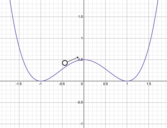
After some amount of time, the ball will come to rest in one of the wells. Which one it is depends a lot on the initial conditions (where it starts and how fast it’s moving) and the damping factor. It’s hard to really measure how accurately the solver is doing with the specific values, but the trend to settle on one side or the other should be plain during testing. The solver is likely either working correctly and approaching one of the two long-term results at +1 or -1, or not really working at all and giving impossible results as time goes on. (Note that altering the timestep may drastically alter the values; this is a very sensitive system.)

Finally, there is the RLC circuit, which is a practical example of a system modeled by differential equations. The signal-flow block model is hopefully sufficient to show how to create the solver if you don’t follow how the circuit works. Here, we can generate a test case using the original values from the text, but we need to know what to expect as output. It turns out there are a few interesting cases to consider, including one that showcases another potential pitfall of numerical methods (not really a problem with streams).

Firstly, here’s a brief explanation of how an RLC circuit works. There are two elements in it that store electrical energy (as charge). The energy stored on a capacitor (the ‘C’) can be measured from its voltage, and on the inductor (the ‘L’) it is a function of its current. These two elements don’t produce any energy on their own, but they don’t consume it either These are ‘ideal’ circuit elements, analagous to frictionless surfaces. If either component has some initial value of voltage or current, the charge will transfer back and forth between them. The voltage on the capacitor will turn into current in the inductor, and vice versa. With just these two components (an ‘LC’ circuit), the oscillation would continue forever. However, the third element of this circuit, which is the resistor R, does nothing but dissipate any energy that passes through it. So when the resistor is part of the circuit, the energy that flows back and forth between the inductor and capacitor decreases a bit at a time until it is totally dissipated by the resistor (as heat).

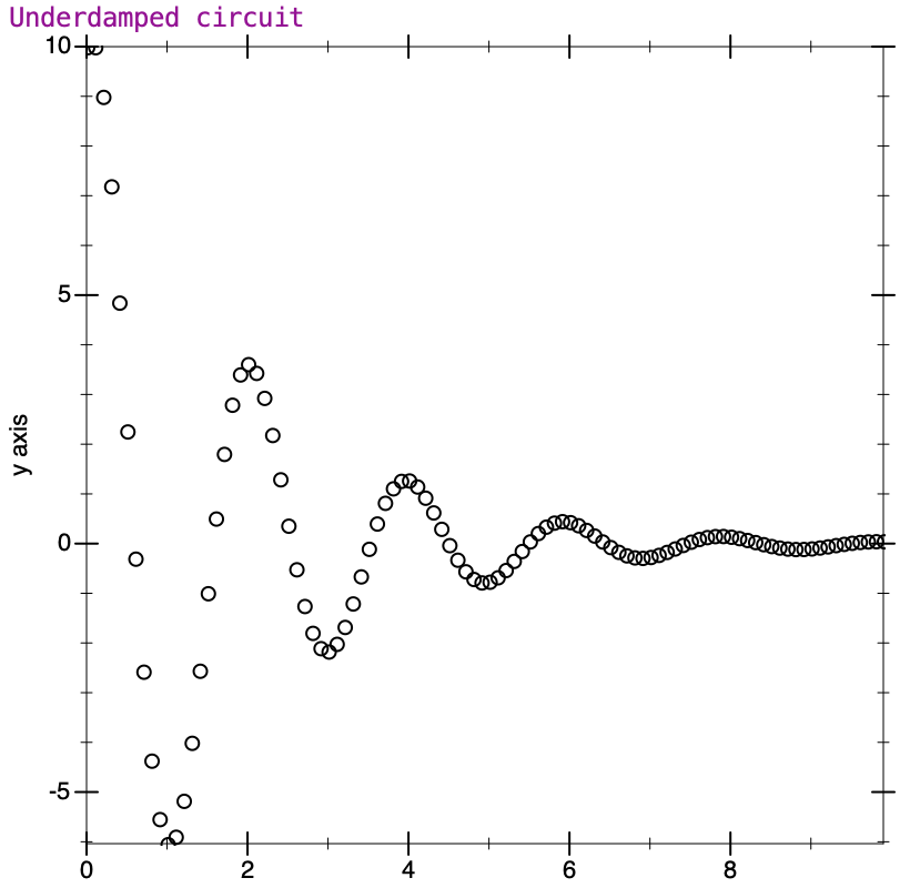
The values given in the example demonstrate the fading oscillation fairly well; the values for both voltage and current go up and down, and decrease in amplitude with each cycle. Here’s what the plot looks like from my runs in Racket.

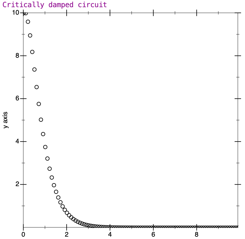
The actual time taken for each ‘cycle’ (from one peak to the next) is determined by the L and C values, and the rate of decrease is determined by the resistor. What happens when the resistor is large enough that the energy is dissipated before the oscillation even starts? Similarly to the Duffing equation, we can define a damping factor (traditionally for this equation zeta [𝜁] is used, not gamma). The damping factor indicates how much relative oscillation will occur. In the situation where 𝜁 = 1, the system is said to be critically damped, and is right at the point where the energy fades just as oscillation is about to start. Here’s the plot of a critically damped system with characteristics similar to the original example.

When the damping factor is lower, we would say the system is underdamped, and some oscillation will always occur. This is the case for the text’s example. If 𝜁 is greater than one, the system is said to be overdamped, and will not oscillate. What is interesting in the overdamped system is that while it goes smoothly toward zero without oscillating (the curve resembles the critically damped case), it takes longer to do so than in the critical case. Circuit designers would need to balance the response time of the system with how much oscillation is acceptable, and choose the damping factor appropriately.

This may have seemed like an unnecessary digression on the workings of this circuit, but I wanted to highlight something about this model. There’s a problem that can arise when we simulate an overdamped case. If the overdamping is very high, and we otherwise use the same simulation parameters from the other cases, we may find that the numbers start to increase without bound. This is not something in the mathematical circuit model per se, or an error with the stream paradigm. The problem is that the timestep might not be appropriate to simulate the changes in the system. In this case, we have to reduce the size of the time step to get correct results.

It is somewhat counterintuitive that the ‘slower’ overdamped system, which doesn’t display a change as rapidly as the others, can have this issue. An issue at the other end of the scale, where a fast oscillation is skipped over when the time step is too large, might be expected (and certainly could happen). Yet, as this demonstrates, problems with numerical methods can creep in regardless of what the scale of the system might seem to be. There are truly a host of issues that are well beyond the scope of this exercise. It’s just worthwhile to know that not all problems are due to faulty procedure implementations.

Stream_353

Exercises 3.5.4.