In the following diagrams, the procedure objects are only shown once, and then omitted in later diagrams. Those procedures are still there. It’s just not really necessary to show them each time, as that part of the diagram does not change. In our model, a procedure (the two-circle symbol with pointers to the parameter list and body, and its enclosing environment) stays stored in memory somewhere and that part of it does not change. When the procedure is evaluated, the bindings determine how the arguments are applied. The stored procedure itself is not modified. Exactly what ‘evaluation’ entails will be a major part of the next chapter; for now, we can consider that the evaluator just reads the stored procedure body and figures out which expression to evaluate next. In most cases I’ve added a box to my diagrams to show which line of the procedure is in the process of being evaluated.

Exercise 3.9.

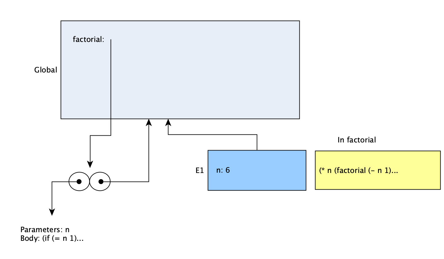
Let’s go over the recursive version first. In the global environment, we start with the procedure factorial defined. We make a call to it with (factorial 6) and a new evaluation frame is created:

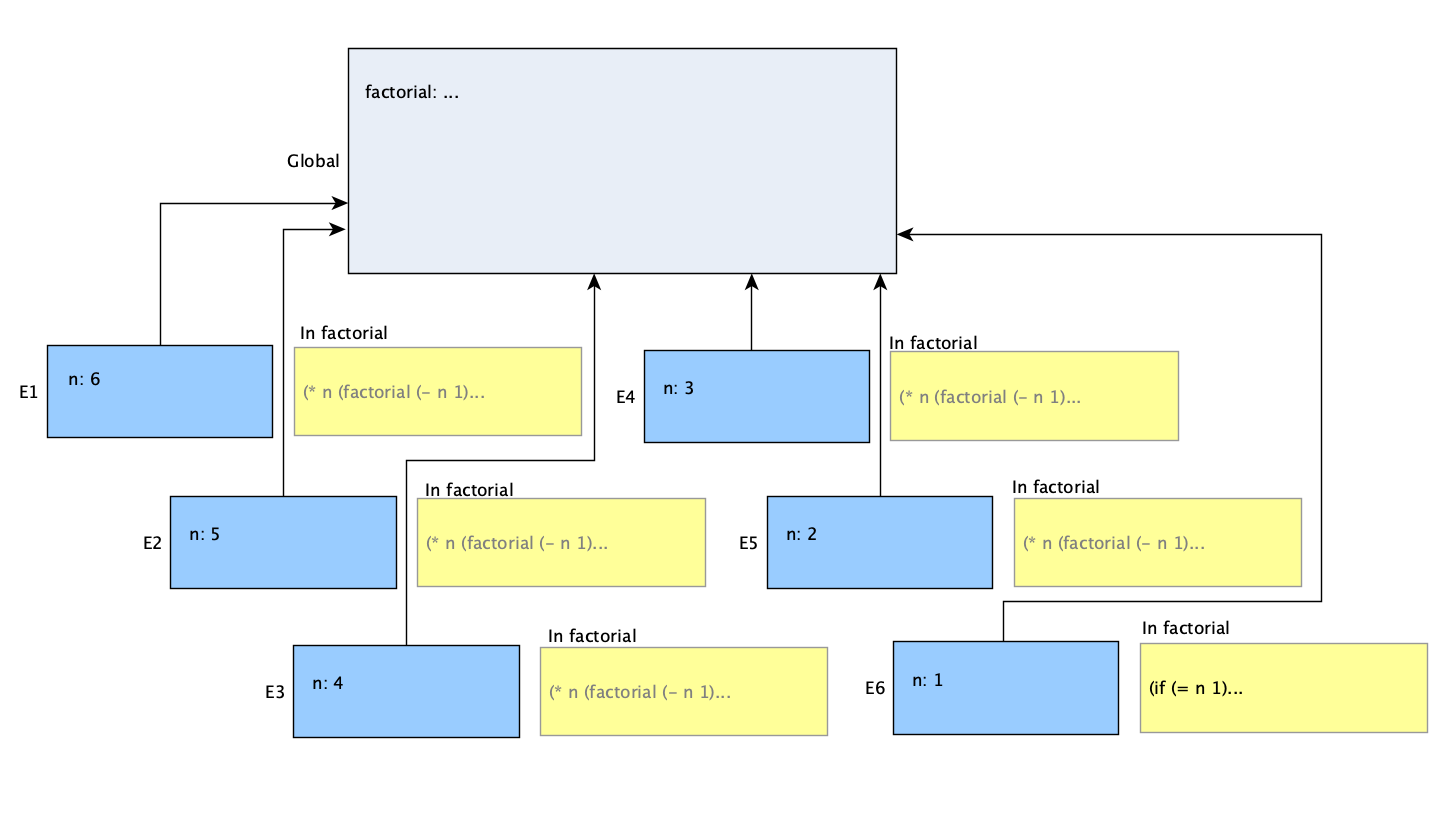
In the course of evaluating (factorial 6), another call to factorial is made. Since factorial is defined in the global environment, the evaluation frame for any call to it is created there as well. This will proceed for each successive call to factorial, all the way to (factorial 1) at the end:

Each procedure is still awaiting the value returned by the procedure calls after it. Once they return, they will finish computing the value and then return. The environment for that call can then be removed, and this will happen in the reverse order in which the environments were created.

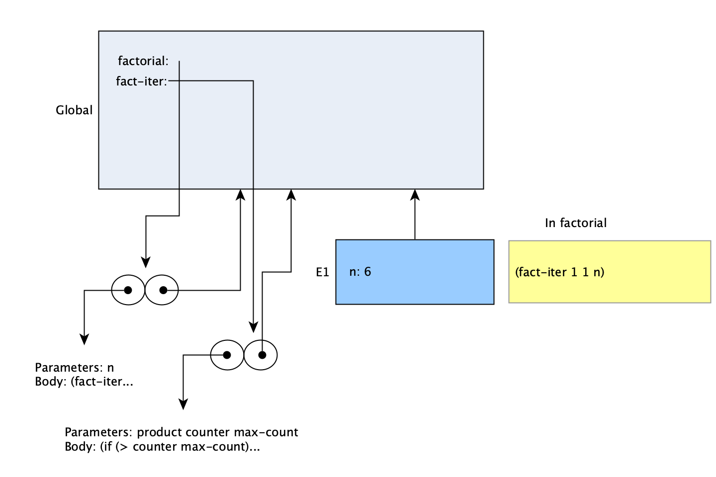
Now, on to the other approach. In the iterative version, there are two procedures defined in the global environment. Otherwise, the model looks initially quite similar to the recursive version, with only the code in the procedure being different:

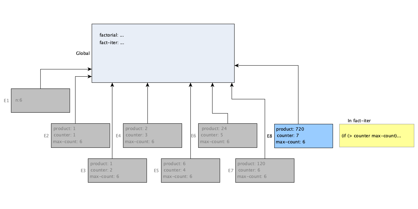
The first procedure calls a second one with different parameters. That means the next frame to be created will be for evaluating fact-iter with the product, counter, and max-count set to their starting values. Each call to fact-iter after that will result in a new call to fact-iter with different arguments, until it is called with counter higher than max-count (the greyed-out environments will be explained shortly):

The repeated calls once again produce new frames in the global environment. That means seven more frames are created. Why seven instead of six, as with the recursive version? That happens because of a slight difference in the way the two versions terminate. The recursive procedure counts down to 1, and then terminates at that point. The iterative version counts up, and does not terminate until the counter is past the maximum. It requires an extra call and thus one more evaluation frame. In total, eight frames are created for the iterative version.

However, as alluded to in the text’s footnote for this exercise, this model doesn’t quite tell the whole story. It turns out that it’s not really necessary for all the environments to be preserved in the iterative version. Each of these calls (save the last one) will do nothing but call a procedure and return the value of that call. Nothing in that environment will be needed again. When that is the case, it’s possible to allow that environment to disappear. It’s for this reason that I’ve grayed out all the frames — it’s not necessary for them to remain, and in fact, the interpreter will remove them. Scheme actually requires their removal The recursive version cannot do this, since each procedure call must wait on the result so it can multiply it by one of its own environment variables before returning.

Under this model, we see that the recursive version grows in space and then shrinks again. The iterative version takes up slightly more space initially, and has more calls (even disregarding the difference in termination conditions), but it never actually requires more than one evaluation frame at a time. This mirrors the substitution model somewhat, which was shown in Figures 1.3 and 1.4 in the text.

There is no ‘solutions’ file for this section, since the procedures are explained in Section 1.2.1 in the text, and there is no real need to verify that they produce this output.